Quantization: What, Why, and How

Quantization is a critical concept in the fields of artificial intelligence (AI) and machine learning (ML), especially as these technologies continue to evolve. This article delves into what quantization is, its necessity, and its impact on AI and ML models.

What is Quantization?

Quantization refers to the process of minimizing the number of bits required to represent a number. In practice, this often involves converting floating-point representations in higher precision formats to lower precision formats. This can include converting an array or weight matrix or model that is in FP32 to FP16, or INT4, or INT8 representations. This process is an essential component of model compression strategies, along with other techniques such as pruning, knowledge distillation, and low-rank factorization.

Why Do We Need Quantization?

The need for quantization arises from several challenges associated with AI and ML models:

1. Size of Models: Contemporary AI models are often large, requiring substantial storage and computational resources for training and inference.

2. Memory and Energy Efficiency: Floating-point numbers, commonly used in AI models, require more memory and are less efficient in terms of energy consumption compared to integer representations.

Benefits of Quantization

1. Improved Inference Speed and Reduced Memory Consumption: Quantization primarily works by converting floating-point numbers to integers. This transformation not only reduces the overall size of the model, making it more compact and storage-efficient, but also significantly enhances the speed of inference.

2. Enhanced Computational Speed: Quantization accelerates computation, particularly during inference, due to the simpler mathematical operations required for integers compared to floating points.

3. Energy Efficiency: With a more compact model size and faster computation, quantization contributes to lower energy consumption.

4. Edge Computing: The reduced size and increased efficiency make it feasible to run sophisticated models on edge devices and smartphones.

Quick Example

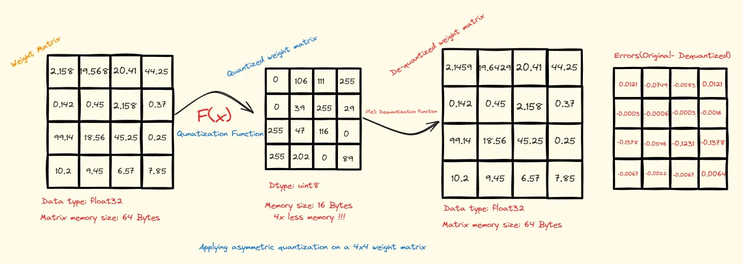
Consider the example illustrated below, where we have a 4x4 weight matrix. These weights are initially stored as 32-bit floating-point numbers, consuming a total of 64 bytes. Our goal is to reduce this footprint while retaining as much of the original information as possible.

import torch

w = [
    [2.158,19.568,20.41,44.25],
    [0.142,0.45,2.158,0.37],
    [99.14,18.56,45.25,0.25],
    [10.2,9.45,6.57,7.85]
    ]
w = torch.tensor(w)

def asymmetric_quantization(weight_matrix, bits, target_dtype= torch.uint8):
    alphas = (weight_matrix.max(dim=-1)[0]).unsqueeze(1)
    betas = (weight_matrix.min(dim=-1)[0]).unsqueeze(1)
    scale = (alphas - betas) / (2**bits-1)
    zero = -1*torch.round(betas / scale)
    lower_bound, upper_bound = 0, 2**bits-1

    weight_matrix = torch.round(weight_matrix / scale + zero)
    weight_matrix[weight_matrix < lower_bound] = lower_bound
    weight_matrix[weight_matrix > upper_bound] = upper_bound

    return weight_matrix.to(target_dtype), scale, zero

def asym_dequant(weignt_matrix,scale,zero):
    return (weignt_matrix-zero)*scale

w_quant,scale,zero = asymmetric_quantization(w, 8)
w_dequant = asym_dequant(w_quant, scale, zero)

print('Original Matrix is: \n',w,'\n\n','Quantized Matrix is: \n',w_quant,'\n\n'\
      'De-quantized is \n',w_dequant,'\n')

original_size_in_bytes= w.numel()*w.element_size()
Qunatized_size_in_bytes= w_quant.numel()*w_quant.element_size()

print(f'Size before quantization: {original_size_in_bytes} \nSize after quantization: {Qunatized_size_in_bytes}')

To achieve compression, we employ a quantization function that maps the original floating-point values to a specified range. In this case, we utilize an asymmetric quantization range of 0-255, corresponding to the uint8 data type.

As a result, the quantized matrix holds values ranging from 0 to 255, and the total memory consumed is now only 16 bytes — a reduction to a quarter of the original size. Furthermore, by applying a dequantization function, we can translate these integers back into floating-point numbers.

Range-Based Linear Quantization

Asymmetric Quantization

In asymmetric quantization, we transform floating-point numbers or vectors from their original range, typically denoted as , into a new, narrower range defined by . Here, represents the bit depth; is the minimum, and is the maximum value within the array or vector.

Let’s examine the formula:

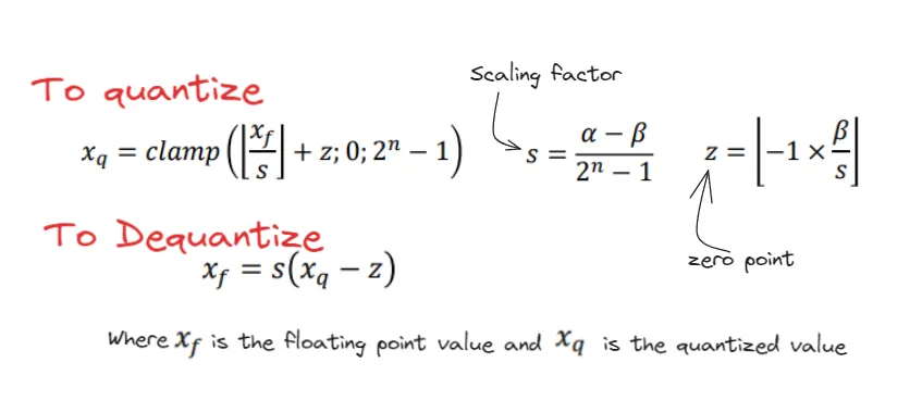
The term is known as the zero point. It maps the zero point from a source vector to an equivalent number in the quantized series. Consider the following example:

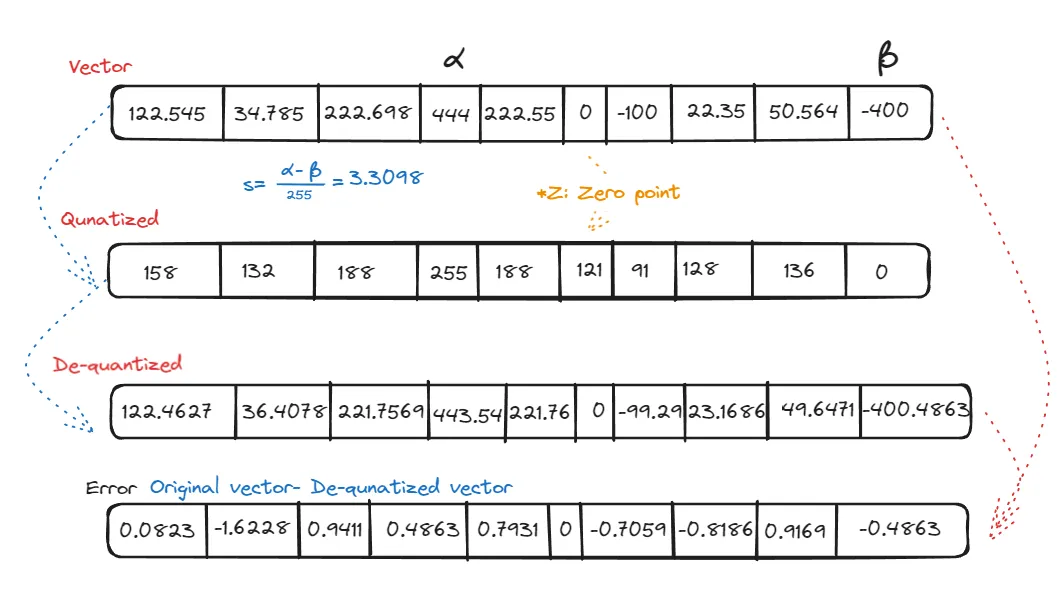
From the example, the number 0 is mapped to 121, which we call the zero point. When we de-quantize, two key parameters come into play: scale and zero point. The scale depends on and , which represent the maximum and minimum values of our vector. However, if any of these points are outliers, they can cause quantization errors.

To tackle this, one strategy is to use percentiles, like the 99th or 10th, for determining the max and min values.

Symmetric Quantization

In symmetric quantization, we map the entire floating-point vector to a range that is equidistant on both sides of the zero point. To determine the mapping range, we first find the maximum absolute value in the vector, which we call . This gives us a mapping range of . Our quantized range then becomes .

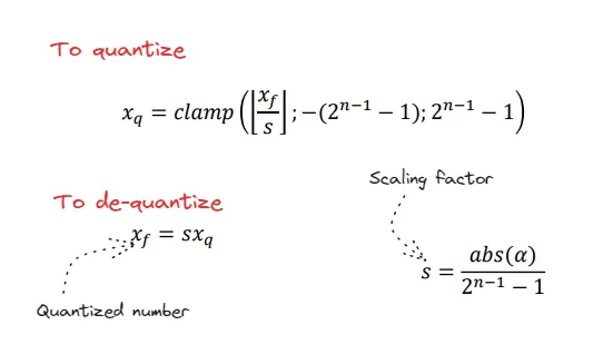
As compared to asymmetric quantization, we don’t have any zero point here — zero is mapped to zero. Let’s consider an example:

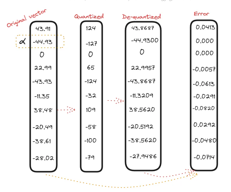
In symmetric quantization, values within the negative domain remain in the negative domain even after quantization. The zero point remains consistent in both vectors.

torch.set_printoptions(sci_mode=False)
def symmetric_quantization(weight_matrix, bits, target_dtype= torch.int8):
    alphas = (weight_matrix.abs().max(dim=-1)[0]).unsqueeze(1)
    scale = (alphas) / ((2**(bits-1))-1)
    lower_bound, upper_bound = -(2**(bits-1)-1), (2**(bits-1))-1

    weight_matrix = torch.round(weight_matrix / scale)
    weight_matrix[weight_matrix < lower_bound] = lower_bound
    weight_matrix[weight_matrix > upper_bound] = upper_bound

    return weight_matrix.to(target_dtype),scale

def symmetric_dequantization(weight_matrix,scale):
    return weight_matrix*scale

w = [[43.91, -44.93,0,22.99,-43.93,-11.35,38.48,-20.49,-38.61,-28.02],
    [56.45,0,125,22,154,0.15,-125,256,36,-365]]

w = torch.tensor(w)

w_quant,scale = symmetric_quantization(w, 8)
w_dequant = symmetric_dequantization(w_quant, scale)

print('Original Matrix is: \n',w,'\n\n','Quantized Matrix is: \n',w_quant,'\n\n'\
      'De-quantized is \n',w_dequant,'\n')

original_size_in_bytes= w.numel()*w.element_size()
Qunatized_size_in_bytes= w_quant.numel()*w_quant.element_size()

print(f'Size before quantization: {original_size_in_bytes} \nSize after quantization: {Qunatized_size_in_bytes}')

Both quantization methods are susceptible to outliers since the scale factor depends on the range. Strategies to mitigate this include using percentile-based range selection or grid search to minimize MSE.

Beyond Linear Quantization

Beyond these, the field of quantization includes methods like DorEfa and WRPN, each offering unique approaches to reducing model size and computational overhead.

Next, we’ll look at Post-Training Quantization (PTQ) and Quantization Aware Training (QAT) — key techniques for making ML models more efficient in production.